Stochastic Processes for Expensive Black-Box Optimization
In this post, we’ll go through one of the techniques of Black-Box Deterministic Optimization: Response Surface Methdology. In general, this approach models the objective and constraint functions with stochastic processes based on a few evaluations at points in the search space; with the goal of predicting the functions’ behavior as we move away from the evaluated points by different amounts in each coordinate direction.
The stochastic process approach has been used in several fields under such names as ‘kriging’, ‘Bayesian optimization’, and ‘random function approach’. It comes with two main advantages:
- Suitability for Expensive Optimization - as it quickly captures the trends over the search space.
- Ease of establishing reasonable stopping rules - as it provide statistical confidence intervals.
Modelling Alternatives
Let’s say we have evaluated a deterministic function, $~y:\mathbb{R}^k\to \mathbb{R}$, at $n$ points. In other words, we have a sample $\mathcal{D}={(x^{(i)},y^{(i)})}_{1\leq i \leq n}$ from the $k$-dimensional space, and we would like to use these observation in guiding our search for the optimal point. Let’s explore possible models that may help us in that.
1. Linear Regression
One can use linear regression as a simple way to fit a response surface to $\mathcal{D}$. In linear regression, the observations are assumed to be generated from the following model.
\begin{equation} y(\mathbf{x}^{(i)}) = \sum_{h} \beta_{h}f_h(\mathbf{x}^{(i)}) + \epsilon^{(i)}\; (i = 1,\ldots,n). \label{eq:lin-reg} \end{equation}
In the above equation, the $f_h(\mathbf{x})$’s are a set of linear or non-linear functions of $\mathbf{x}$; the $\beta_h$’s are unknown parameters of the model to be estimated; and the $\epsilon^{(i)}$’s are independent error terms with a normal distribution of zero mean and $\sigma^2$ variance.
Employing Eq. \ref{eq:lin-reg} has two main concerns:
- A Conceptual Concern: Our function $f$ is deterministic. Therefore, any improper fit of Eq. \ref{eq:lin-reg} will be a modelling error—i.e., incomplete regression term $\sum_{h} \beta_{h}f_h(\mathbf{x}^{(i)})$—rather than measurement noise or error—i.e., the $\epsilon^{(i)}$ term. In essence $\epsilon^{(i)}=\epsilon(\mathbf{x}^{(i)})$ captures the value of the left-out regression terms at $\mathbf{x}^{(i)}$. And if $y(\mathbf{x})$ is continuous, then $\epsilon(\mathbf{x})$ is continuous as well. Thus, if two points $\mathbf{x}^{(i)}$ and $\mathbf{x}^{(j)}$ are close, then the errors $\epsilon(\mathbf{x}^{(i)})$ and $\epsilon(\mathbf{x}^{(j)})$ should be close as well.
- A Practical Concern: How to define the $f_h$’s functions. Indeed, if we knew the perfect form of Eq. \ref{eq:lin-reg}, our function $f$ would not have been a black box in the first place. One can certainly employ a meta-model $($some referred to it as flexible functional form$)$ approach to decide the most suitable form of Eq. \ref{eq:lin-reg}. However, this approach comes with an additional set of parameters $($hyperparameters$)$ and requires many more function evaluations.
In light of the above concerns, it makes no sense to assume that the error terms $\epsilon^{(i)}$’s are independent. Alternatively, we can assume that these terms are associated / related and that the level of such association $($correlation$)$ is low when the corresponding points $\mathbf{x}^{(i)}$’s are far away and high when they are close. The following equation captures this assumption of correlation.
\begin{equation} Corr[\epsilon(\mathbf{x}^{(i)}),\epsilon(\mathbf{x}^{(j)})] = \exp\big(- \sum_{h=1}^{k} \theta_h |x^{(j)}_h-x^{(j)}_h|^{p_h}\big)\;, \theta_h \geq 0\;, p_h \in [0,1]\;. \label{eq:corr-fct} \end{equation}
The parameters $\theta_h$’s and $p_h$’s controls how fast the degree of correlation changes between two errors terms as the (weighted) distance between the corresponding points changes as shown in the figure below. In general, $\theta_h$ measures the importance / activity of the $h^{th}$ variable $x_h$ $($the higher $\theta_h$ is, the faster the correlation drops as the corresponding points move away in the coordinate direction $h)$, while $p_h$ captures the function smoothness in the coordinate direction $h$ $(p_h$ = 2 is for smooth functions$)$.
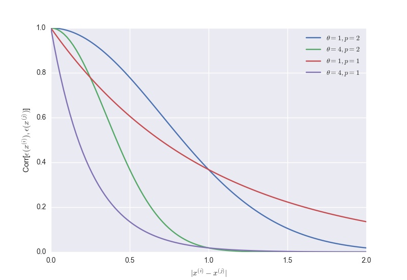
Figure 1. Correlation Function $($Eq. \ref{eq:corr-fct}$)$ with different parameters.
Having modelled the correlation between our observations, fitting the regression term to our observations is less of a concern now. In fact, this forms the basis of the stochastic process model presented next.
2. DACE $($Design and Analysis of Computer Experiments [1]$)$
Based on the correlation model $($Eq. \ref{eq:corr-fct}$)$, one can view the error term $\epsilon(\mathbf{x})$ as a stochastic process - a set of correlated random variables indexed by the $k$-dimensional space of $\mathbf{x}$. Therefore, the observations can be modeled with the following stochastic process:
\begin{equation} y^{(i)} = \mu + \epsilon(\mathbf{x}^{(i)})\; (i=1, \ldots, n). \label{eq:dace} \end{equation}
In comparison to Eq. \ref{eq:lin-reg}, $\mu$ $($the mean of the stochastic process$)$ is the simplest regression term $($ a constant $)$; $\epsilon(\mathbf{x}^{(i)})\sim \mathcal{N}(0, \sigma^2)$ with a correlation given by Eq. \ref{eq:corr-fct}. This model is commonly referred to as DACE - an acronym to the paper that popularized it [1].
We can estimate DACE’s $2k+2$ parameters by maximizing the likelihood of our sample $\mathcal{D}$. With the correlation between two error terms defined as above, the vector $\mathbf{y}=[y^{(1)},\ldots, y^{(n)}]$ of observed function values is a normal random $n$-vector. That is, $\mathbf{y}\sim\mathcal{N}(\mu, \sigma^2\mathbf{R})$. Thus, the likelihood function of our samples can be written as follows.1 \begin{equation} f(\mathbf{y};\theta,p, \mu, \sigma) = \frac{1} {(2\pi)^{n/2}(\sigma^2)^{n/2}|\mathbf{R}|^{(1/2)}} \exp\big(-\frac{(\mathbf{y}-\mathbf{1}\mu)^{T} \mathbf{R}^{-1} (\mathbf{y}-\mathbf{1}\mu)}{2\sigma^2}\big) \label{eq:likelihood} \end{equation}
Eq. $\ref{eq:likelihood}$ can be optimized with respect to $\mu$ and $\sigma^2$ in closed form by taking the partial derivative of its log:
The above equations can in turn be plugged into the likelihood function to form a concentrated likelihood function, which can be optimized with resepct to the parameters $\theta_h$’s and $p_h$’s. Subsequently, the corresponding values of $\hat{\mu}$ and $\hat{\sigma}^2$ are computed.
Having estimated the parameters of our stochastic process model, we can now use it to predict the function value at new points in the $k$-dimensional space. The stochastic process model encodes the left-out terms of the regression model using the correlated errors. In other words, these correlated errors must be employed to adjust the prediction above or below the constant regression term $\hat{\mu}$. To see how this can be done, assume that we are interested in predicting the function value at $x^{(n+1)}$ and let $y^{*}$ be some prediction candidate for $f(x^{(n+1)})$. To measure how well $(x^{(n+1)},y^{*})$ fits the sample $\mathcal{D}$, one can compute the joint $($augmented$)$ likelihood function of $\tilde{\mathbf{y}} = (\mathbf{y}\; y^{*})$ - $f(\tilde{\mathbf{y}};\theta,p, \hat{\mu}, \hat{\sigma})$ from Eq. \ref{eq:likelihood}’s $f(\mathbf{y};\theta,p, \mu, \sigma)$. Taking the log of Eq. \ref{eq:likelihood}, it is easy to see that the only term that depends on $y^{*}$ is $(\tilde{\mathbf{y}}- \mathbf{1}\hat{\mu})^{T}{\tilde{\mathbf{R}}}^{-1}(\tilde{\mathbf{y}}- \mathbf{1}\hat{\mu})$ with , where $\mathbf{r} = \mathbf{r}(\mathbf{x}^{(n+1)}) = [Corr[\epsilon(\mathbf{x}^{(1)}),\epsilon(\mathbf{x}^{(n+1)})],\ldots,Corr[\epsilon(\mathbf{x}^{(n)}),\epsilon(\mathbf{x}^{(n+1)})]]$.
Applying the blockwise inversion formula on $(\tilde{\mathbf{y}}- \mathbf{1}\hat{\mu})^{T}{\tilde{\mathbf{R}}}^{-1}(\tilde{\mathbf{y}}- \mathbf{1}\hat{\mu})$, we have:
Thus, setting the derivative of the above term with respect to $y^{*}$ to zero gives the best prediction’s formula at $\mathbf{x}^{(n+1)}$ that fits the sample $\mathcal{D}$ as follows.
\begin{equation} \hat{y}(\mathbf{x}) = \hat{\mu} + {\mathbf{r}(\mathbf{x})}^{T}\mathbf{R}^{-1}(\mathbf{y}-\mathbf{1}\hat{\mu}) \label{eq:prediction} \end{equation}
While this value maximizes the joint augmented likelihood of $(x^{(n+1)},y^{*})$ and $\mathcal{D}$, it is interesting to note that it also corresponds to the mean of the normal probablity density function of the function value at $x^{(n+1)}$ conditioned on $\mathcal{D}$.
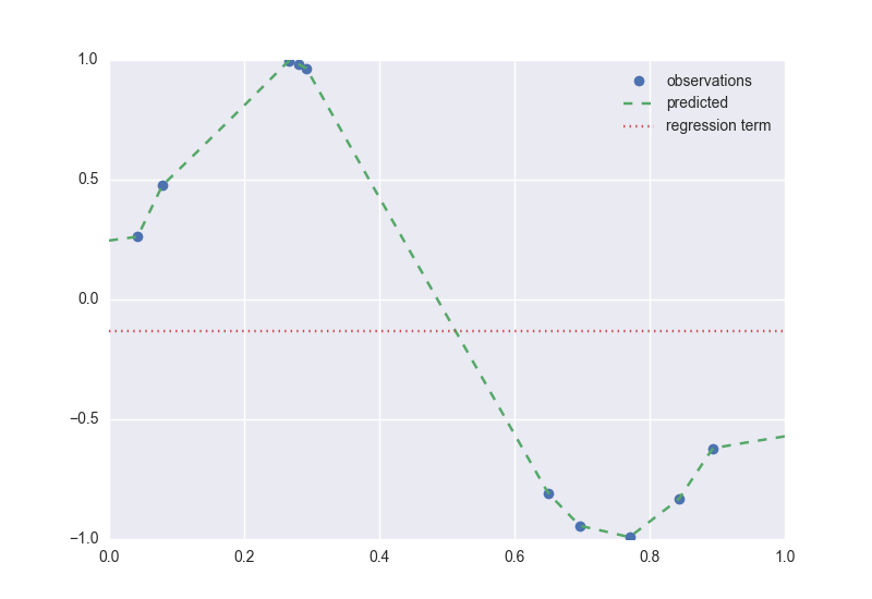
Figure 2. Application of Eq. \ref{eq:prediction}
Figure 2 shows predicted values of $f$ at different points according to Eq. \ref{eq:prediction}. DACE’s predictor $($Eq. \ref{eq:prediction}$)$ is also an interpolator of $\mathcal{D}$. That is $\hat{y}(\mathbf{x}^{(i)}) = \hat{\mu} + {\mathbf{r}(\mathbf{x}^{(i)})}^{T}\mathbf{R}^{-1}(\mathbf{y}-\mathbf{1}\hat{\mu}) = y^{(i)}$, since ${\mathbf{r}(\mathbf{x}^{(i)})}^{T}\mathbf{R}^{-1}={(\mathbf{R}^{-1}\mathbf{R}_i)}^{T}=\mathbf{e}^T_i$. Furthermore, the prediction accuracy can be characterized by the mean squared error, which can be proved to be as follows.2
TO BE COMPLETED…
References
This post is based on the following papers:
-
Sacks, Jerome, et al. Design and analysis of computer experiments. Statistical science $($1989$)$: 409-423.
-
Jones, Donald R.; Schonlau, Matthias; Welch, William J. Efficient global optimization of expensive black-box functions. J. Global Optim. 13 $($1998$)$, no. 4, 455–492.