Benchmarking Open-Source Bayesian Optimization Implementations on the COCO Noiseless Testbed
There have been several open-source implementations of Bayesian Optimization algorithms. In this post, we evaluate a couple of them $($tabulated in the table below$)$ on the COCO benchmark platform.
| Implementation | Source |
|---|---|
| SkGP | https://github.com/scikit-optimize/scikit-optimize/ |
| SkGBRT | https://github.com/scikit-optimize/scikit-optimize/ |
| GPyOptimize | http://sheffieldml.github.io/GPyOpt/ |
| BO | https://github.com/fmfn/BayesianOptimization |
| PyBO | https://github.com/mwhoffman/pybo |
| YelpMOE | https://github.com/Yelp/MOE/ |
| HyperOpt | http://hyperopt.github.io/hyperopt/ |
| Spearmint | https://github.com/HIPS/Spearmint |
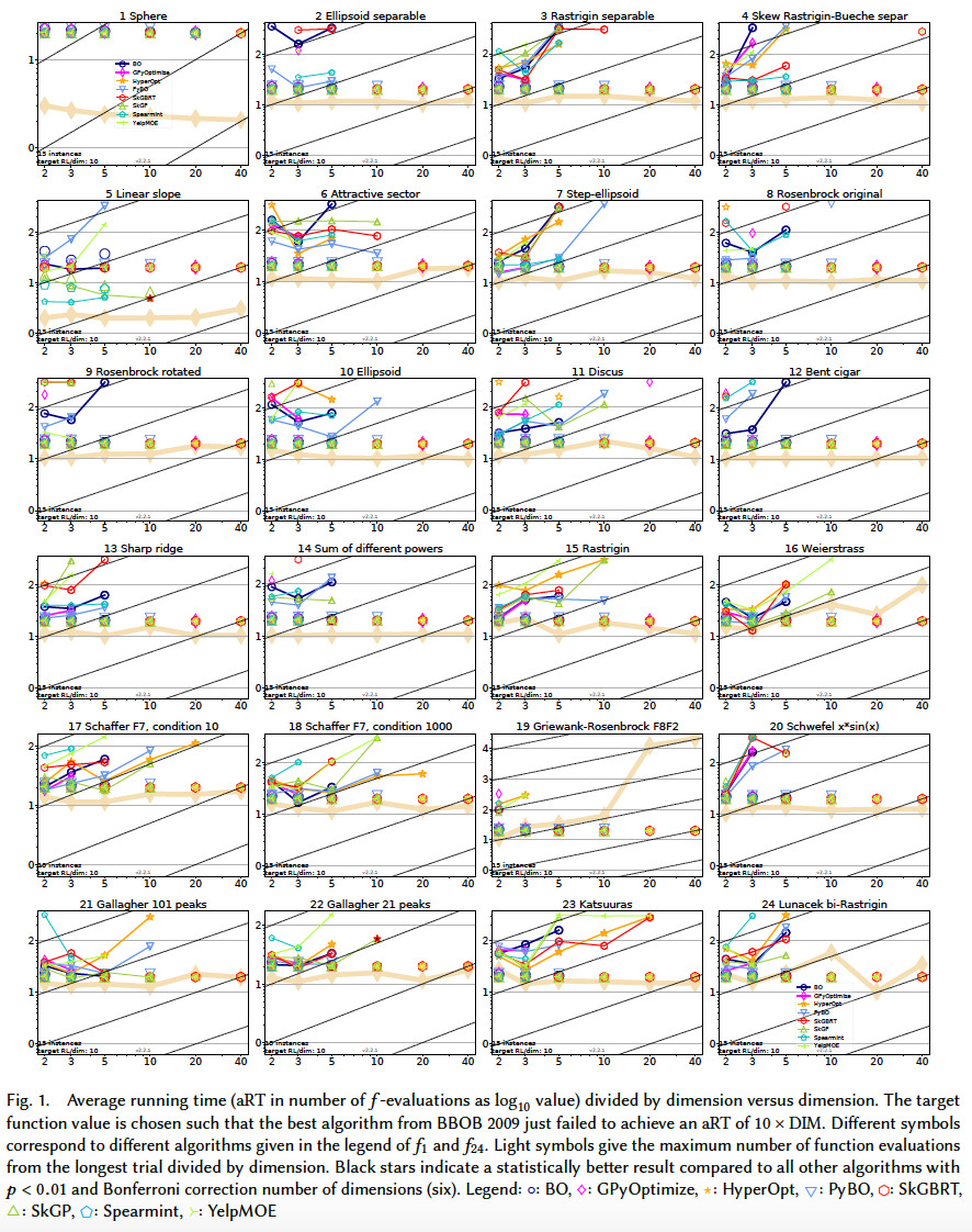
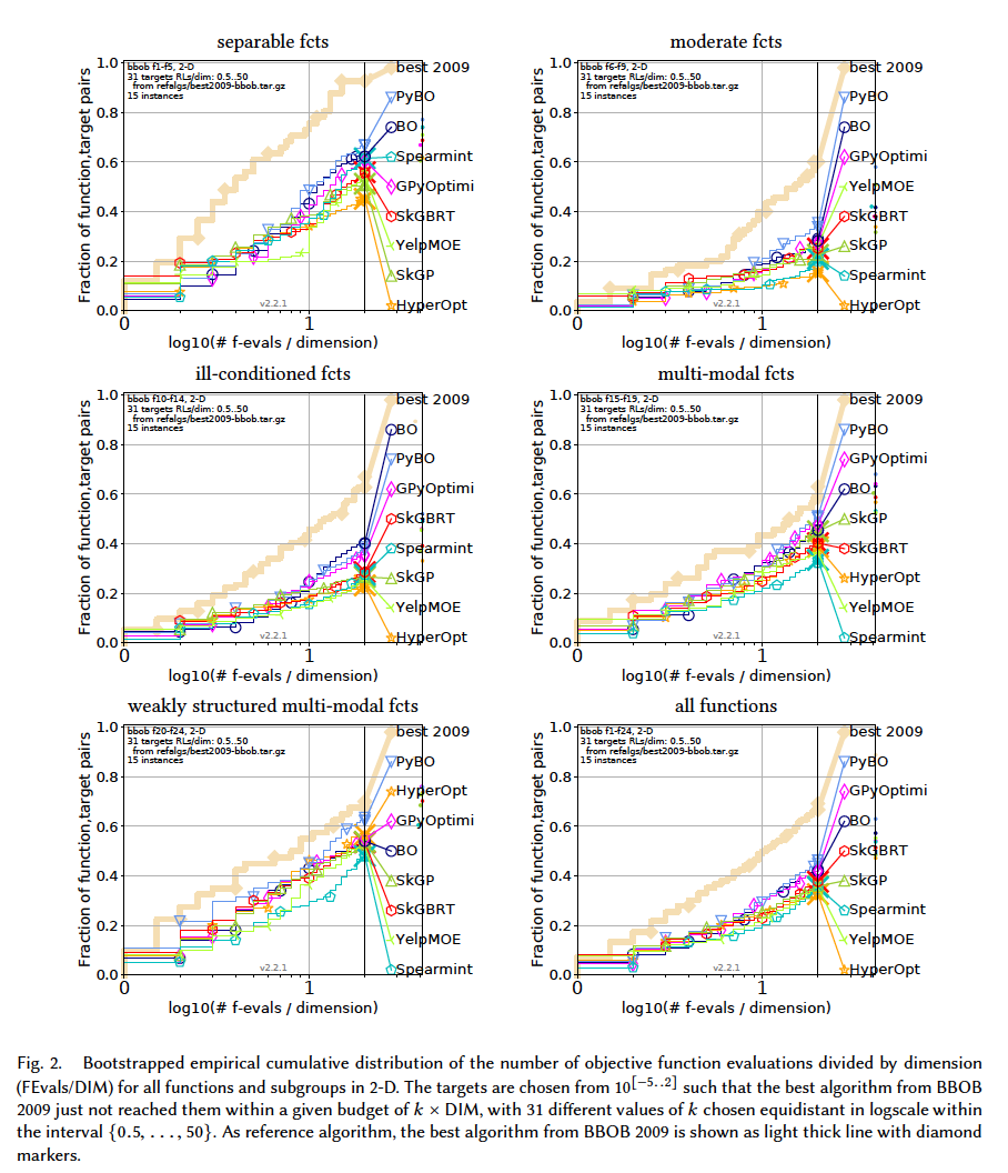
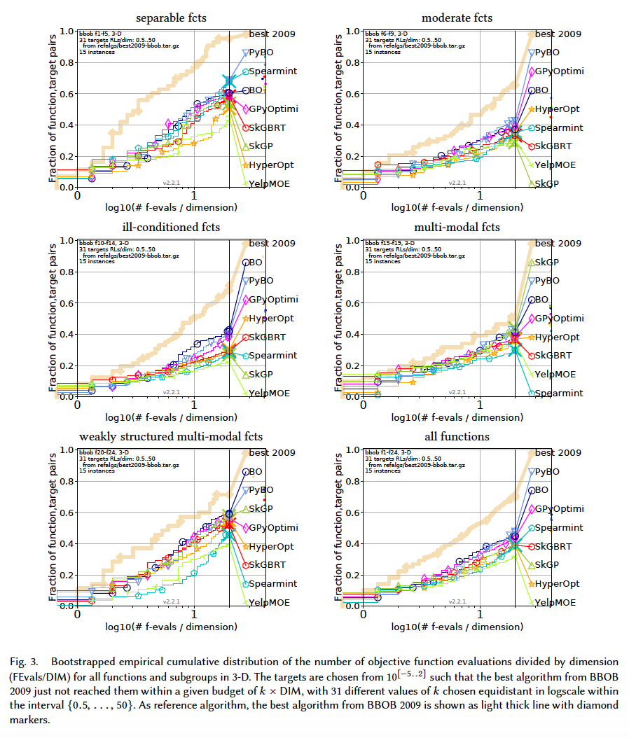
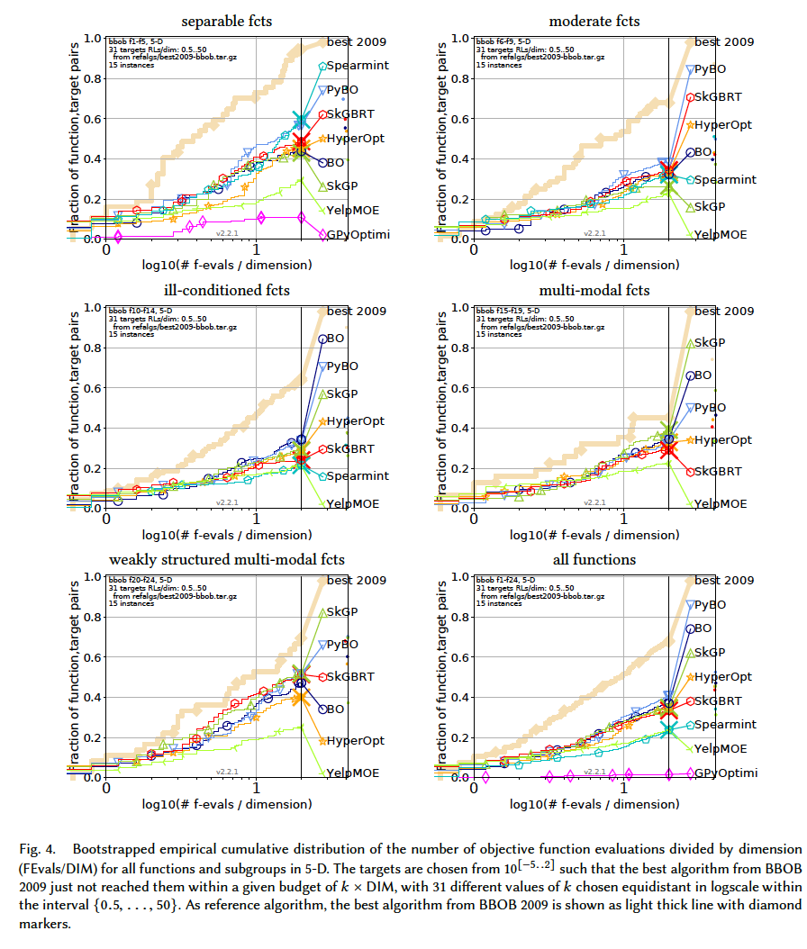
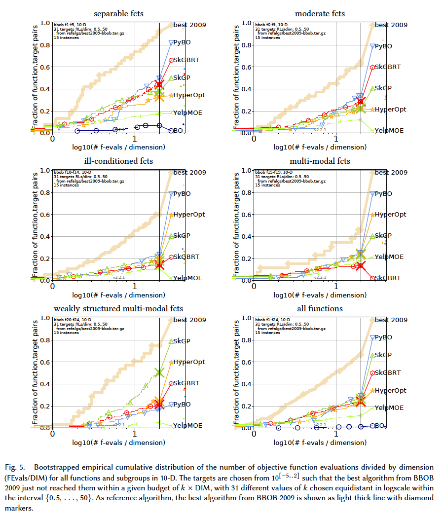
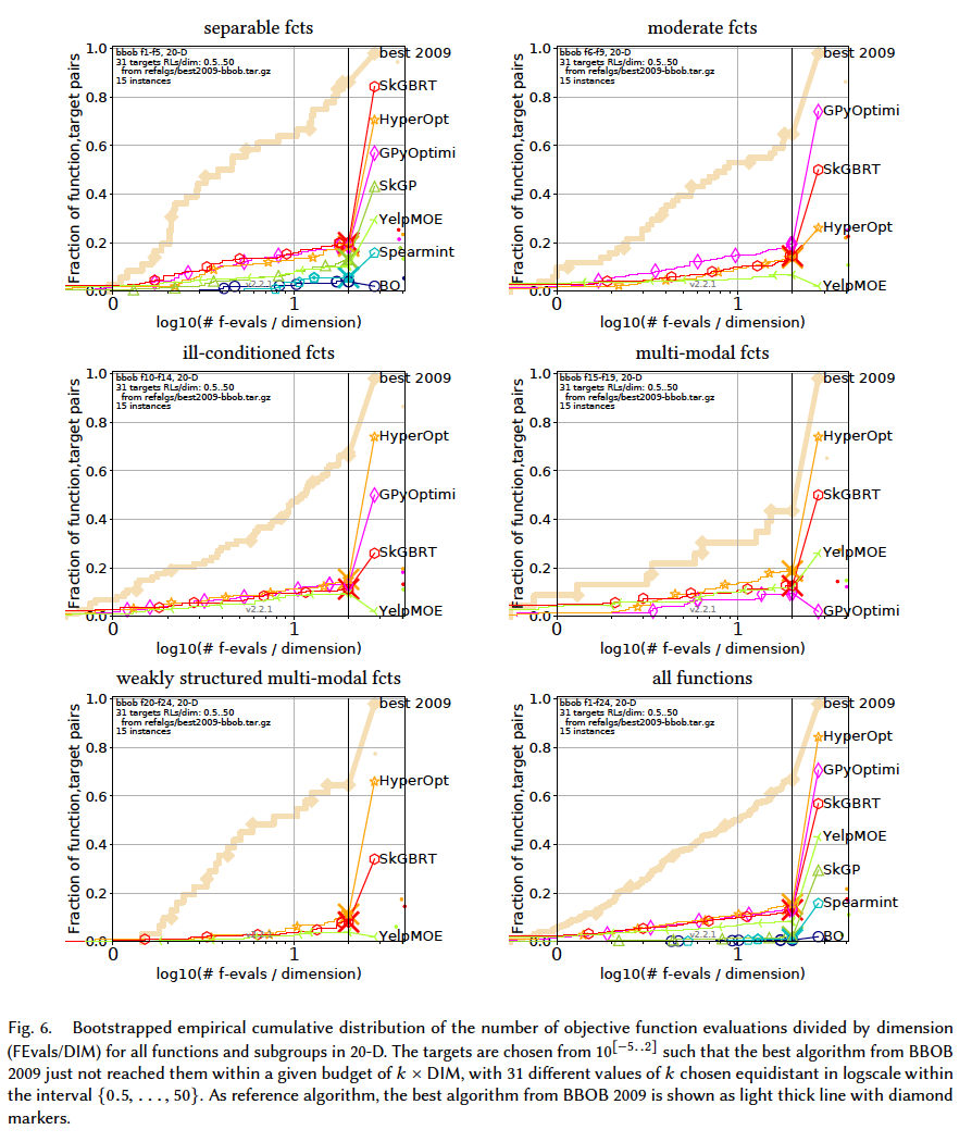
Results from experiments according to [6] and [2] on the benchmark functions given in [1, 5] are presented in the figures below. The experiments were performed with COCO [4], version 2.0, with an evaluation budget of 20 times the problem dimensionaliy.
The average runtime (aRT), used in the figures and tables, depends on a given target function value, $f_t = f_{opt} + \triangle f$ , and is computed over all relevant trials as the number of function evaluations executed during each trial while the best function value did not reach $f_t$, summed over all trials and divided by the number of trials that actually reached $f_t$ [3, 7].
In terms of running time, from slowest to fastest: GPyOptimize, Spearmint, BO, PyBO, SkGP, YelpMOE, SKGBRT, HyperOpt.
In terms of performance, in low-dimension $(D\leq 10)$, PyBO appears to be outperforming consistently. With higher dimensions, most of the algorithms get extremely slow and algorithms like SkGP and SkGBRT seem to be a good tradeoff.
Note: The figures about 20-D and 40-D $($ and even 10-D to some extent $)$ should be considered carefully. Not all the algorithms manage to solve the probelms at the time of producing the results. E.g., Spearmint manages to solve 20-D separable functions, while the rest of the problems are not solved $($ can you see its curve is present in the separable fcts subplot but not the rest $)$. This in turn, affects its final standing in the all fcts subplot. The 2-D and 3-D plots are the only ones in which all the algorithms manage to solve all the problems.
- S. Finck, N. Hansen, R. Ros, and A. Auger. 2009. Real-Parameter Black-Box Optimization Benchmarking 2009: Presentation of the Noiseless Functions. Technical Report 2009/20. Research Center PPE. hp://coco.lri.fr/downloads/download15.03/bbobdocfunctions.pdf Updated February 2010.
- N. Hansen, A Auger, D. Brockho, D. Tuˇsar, and T. Tuˇsar. 2016. COCO: Performance Assessment. ArXiv e-prints arXiv:1605.03560 (2016).
- N. Hansen, A. Auger, S. Finck, and R. Ros. 2012. Real-Parameter Black-Box Optimization Benchmarking 2012: Experimental Setup. Technical Report. INRIA. hp://coco.gforge.inria.fr/bbob2012-downloads
- N. Hansen, A. Auger, O. Mersmann, T. Tuˇsar, and D. Brockho. 2016. COCO: A Platform for Comparing Continuous Optimizers in a Black-Box Seing. ArXiv e-prints arXiv:1603.08785 (2016).
- N. Hansen, S. Finck, R. Ros, and A. Auger. 2009. Real-Parameter Black-Box Optimization Benchmarking 2009: Noiseless Functions Denitions. Technical Report RR-6829. INRIA. hp://coco.lri.fr/downloads/download15.03/bbobdocfunctions.pdf Updated February 2010.
- N. Hansen, T. Tuˇsar, O. Mersmann, A. Auger, and D. Brockho. 2016. COCO: e Experimental Procedure. ArXiv e-prints arXiv:1603.08776 (2016). [7] Kenneth Price. 1997. Dierential evolution vs. the functions of the second ICEO. In Proceedings of the IEEE International Congress on Evolutionary Computation. IEEE, Piscataway, NJ, USA, 153–157. DOI:hp://dx.doi.org/10.1109/ICEC.1997.592287