Computing the Optimal Discriminator between Mixture of Gaussians
Let $p$ and $q$ be two mixtures of $k$ univariate Gaussians as follows:
We are interested in a discriminator $D$ that distinguishes between the above distributions. Let’s assess $D$’s performance with the WGAN objective
That is, the greater $L$ is, the better our discriminator $D$ is. Let the output range of $D$ be $[0,1]$. $L(D)$ can be written as
Since $D(x)\geq 0$, $L(D)$ is maximized with $D(x)=0$ for $p(x)<q(x)$ and $D(x)=1$ for $p(x)\geq q(x)$. With this observation at hand, one can think of the discriminator as an indicator function, with the optimal one being $D^*(x)=\mathbb{1}{p(x)\geq q(x)}$.
For univariate Gaussians, $D^*(x)=1$ on interavls where $p(x)\geq q(x)$ and $0$ otherwise. To find these intervals, one can look for the zero-crossings of the function $p(x)-q(x)$. From Theorem A.2, the linear combination $p(x)-q(x)$ has at most $2k-1$ zero-crossings.
With $k=2$, we have 3 zero-crossings, which we can find with a root-finding solver given good initial guesses. Subsequently, $p(x)\geq q(x)$ over at most $2k-2=2$ disjoint intervals. What’s left now is computing the lower and upper bounds of these intervals for an optimal discriminator. We will demonstrate this in the following snippets.
import numpy as np
import matplotlib.pyplot as plt
from scipy.optimize import root
from scipy.stats import norm


def f(_x, *args):
	"""
	evaluate p(x) - q(x)
	It is assumed that sigma = 1 for all the Gaussians
	"""
    _params = args[0]
    p_x = 0.5 * (norm.pdf(_x, loc=_params['p_mu_1']) + norm.pdf(_x, loc=_params['p_mu_2']))
    q_x = 0.5 * (norm.pdf(_x, loc=_params['q_mu_1']) + norm.pdf(_x, loc=_params['q_mu_2']))
    return p_x - q_x


def solve_fx(_f, x0, _params):
	"""
		Find the zero crossing
	"""
    _res = root(_f, x0, _params)
    return float(_res.x)

def get_optimal_bounds(params):
	"""
		computes the optimal bounds
	"""
    sorted_param_names = sorted(params, key=params.get)

    x = np.linspace(params[sorted_param_names[0]], params[sorted_param_names[-1]], 1000)
    y = f(x, params)

    crosses = np.where(np.diff(np.sign(y[y != 0])))[0]
    positives = np.where(y >= 0)[0]

    x0s = x[crosses]
    res = root(f, x0s, params)

    vals = list(res.x)

    if len(vals) == 1:
        if y[crosses[0]] > 0:
            l_1 = - np.float("inf")
            r_1 = vals[0]
            l_2 = r_1
            r_2 = l_2
        else:
            l_1 = vals[0]
            r_1 = vals[0]
            l_2 = vals[0]
            r_2 = np.float("inf")
    elif len(vals) == 2:
        if y[crosses[0]] > 0:
            l_1 = - np.float("inf")
            r_1 = vals[0]
            l_2 = vals[1]
            r_2 = np.float("inf")
        else:
            l_1 = vals[0]
            r_1 = 0.5 * (vals[0] + vals[1])
            l_2 = r_1
            r_2 = vals[1]
    elif len(vals) == 3:
        if y[crosses[0]] > 0:
            l_1 = - np.float("inf")
            r_1 = vals[0]
            l_2 = vals[1]
            r_2 = vals[2]
        else:
            l_1 = vals[0]
            r_1 = vals[1]
            l_2 = vals[2]
            r_2 = np.float("inf")
    elif len(vals) == 0:
        # any arbitrary value
        l_1, r_1, l_2, r_2 = -10., 0., 0., 10.
    else:
        raise Exception("There should be at most 3 crossings!")

    return l_1, r_1, l_2, r_2
Let’s visulaize an arbitrary set of intervals, note here we have two mixture of 2 Gaussian, that is there exist at most 3 zero crossings.
# viz intervals for D(x) =  1{-3<=x<= -1} | 1{1<=x<=3}
plot_bounds([-3, -1, 1, 3],
            {'p_mu_1': -2, 'p_mu_2': 2, 'q_mu_1': 1, 'q_mu_2': 5})
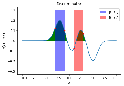
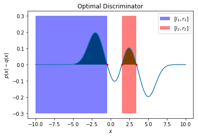
The bounds are covering regions where $p(x) < q(x)$, this should not be the case for an optimal discriminator $D^*(x)$ as shown below.
# viz opt disc bounds D^*(x)
params = {'p_mu_1': -2, 'p_mu_2': 2, 'q_mu_1': 1, 'q_mu_2': 5}
plot_opt_disc(params)