On DeepMind's Population-Based Training
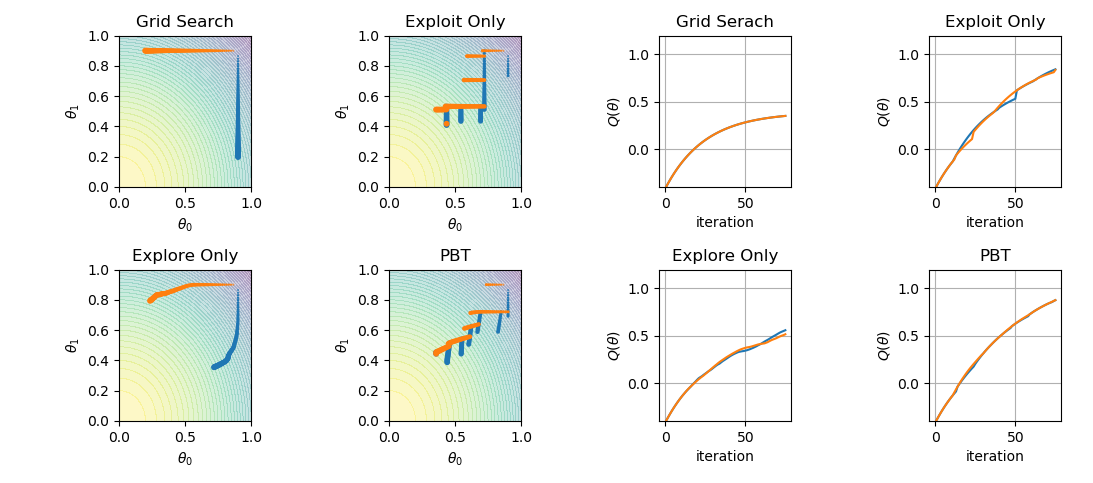
DeepMind has recently released a paper about population-based training of neural nets. The proposition is a simple asynchronous optimization algorithm, which jointly optimizes a population of models and their hyperparameters. In this post, I aim to demonstrate a simple implementation of the algorithm by reproducing the paper’s Figure 2.

The objective is to maximize the function
def q(theta):
    return 1.2 - np.sum(np.array(theta)**2)
Think of the above function as the validation set performance whose closed-form expression is unknown. However, we can still query its value $($ evaluate $)$ at specific $\theta$. While our goal is to maximize it and achieve a model with good generalization capabilities, we optimize our neural model $($ tune its parameters $)$ with respect to the training set performance. That is, our model is optimized w.r.t. to a surrogate objective $\hat{Q}$ function rather than the objective function we are after.
In an ideal setup, one would like $\hat{Q}=Q$ $($ or at least optimizing $\hat{Q}$ should correspond to optimizing $Q$ as well$)$, but this is not the case in general. The quality of this approximation $($or coupled optimization $)$ is often dependent on the model at hand and how we are training it: the hyperparameters. In other words, when we optimize $\hat{Q}$ w.r.t. $\theta$, we are doing so given $($ conditioned on $)$ a set of hyperparameters, $\hat{Q}(\theta\mid h)$.
In the considered toy example, let the mpirical loss / training set performance by parameterized by $h$ as follows.
def q_hat(theta, h):
    # this is used by `step` function to perform
    # gradient updates
    return 1.2 - np.sum(np.dot(np.array(h), np.array(theta)**2))
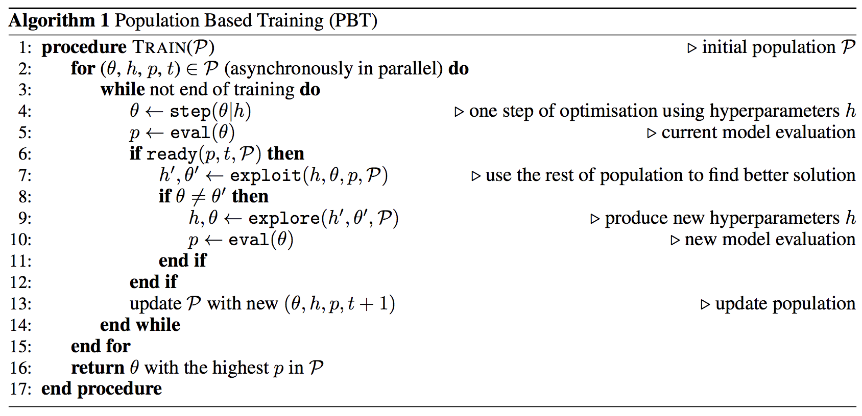
The task now boils down to using $\hat{Q}$ to tune $\theta$ while searching for $h$ to make the tuning process as efficient as possible in $($ indirectly $)$ optimizing $Q$. PBT is one solution to do so. Here is the pesudocode, and below is an implementation of the same.

Let’s start with modeling the population members:
class Member(object):
    def __init__(self, theta=[0., 0.], h=[0., 0.], _id=1, _eta=0.01, _sigma=1e-1):
        self.theta = theta
        self.h = h
        self.id = _id
        self.num_steps = 0
        self.p = q(self.theta)
        self._eta = _eta
        self._sigma = _sigma
        ## for visualization
        self.trace = []
        self.ps = [self.p]

    def eval(self):
        self.p = q(self.theta)

    def ready(self):
        return self.num_steps > 10

    def step(self):
        for i in range(2):
            self.theta[i] +=  self._eta * (-2. * self.h[i] * self.theta[i])
        self.num_steps += 1

    def explore(self):
        for i in range(2):
            self.h[i] = np.clip(self.h[i] + self._sigma * np.random.randn(), 0, 1)

    def exploit(self, other):
        if self.p <= other.p:
            self.theta = list(other.theta)
            self.p = other.p
            self.num_steps = 0
            return True
        else:
            return False

    def log(self):
        self.trace.append(list(self.theta))
        self.ps.append(self.p)

    def __str__(self):
        return 'theta:' + '%.2f' % self.theta[0] + ',%.2f' % self.theta[1] + \
               '| h:' + '%.2f' % self.h[0] + ',%.2f' % self.h[1] + '| id' + str(self.id) + \
               '| p:' + '%.2f' % self.p + '| steps:' + str(self.num_steps)
Here’s PBT implementation. I’ve put flags to show PBT in explore, exploit, grid search modes.
def pbt(grid=False, explore_only=False, exploit_only=False):
    # a check to ensure only one mode is selected for PBT
    assert grid + exploit_only + explore_only <= 1, "at most one flag can be set for PBT modes"
    # init population
    population = [
        Member(theta=[0.9, 0.9], h=[0,1], _id=0),
        Member(theta=[0.9, 0.9], h=[1,0], _id=1)
        ]
    member_ids = np.arange(len(population))
    # begin training
    for _ in range(75):
        np.random.shuffle(member_ids)
        for mem_id in member_ids:
            member = population[mem_id]
            member.step()
            member.eval()
            if member.ready() and not grid:
                if explore_only:
                    member.explore()
                else:
                    member.exploit(population[(mem_id + 1) % 2])
                    if not exploit_only:
                        member.explore()
                    member.eval()
            member.log()

    traces = [population[i].trace for i in range(len(population))]
    ps = [population[i].ps for i in range(len(population))]
    return traces, ps
Let’s plot the four modes
f, axes = plt.subplots(2, 4)#, sharex=True)

traces, ps = pbt(grid=True)
plot_traces(axes[0,0], traces, title='Grid Search')
plot_curves(axes[0,2], ps, title='Grid Serach')

traces, ps = pbt(exploit_only=True)
plot_traces(axes[0,1], traces, title='Exploit Only')
plot_curves(axes[0,3], ps, title='Exploit Only')

traces, ps = pbt(explore_only=True)
plot_traces(axes[1,0], traces, title='Explore Only')
plot_curves(axes[1,2], ps, title='Explore Only')

traces, ps = pbt()
plot_traces(axes[1,1], traces, title='PBT')
plot_curves(axes[1,3], ps, title='PBT')

plt.tight_layout()
plt.show()
which results in the following:
