A Gentle Tour through Sampling Techniques

In this post, we’ll take a quick tour into the sampling world and how it might be handy in some applications. Let’s start with some setup code.

import numpy as np
import pandas as pd
import numpy.random as rnd
import seaborn as sns
import scipy
from mpl_toolkits.mplot3d import Axes3D
%pylab inline

Populating the interactive namespace from numpy and matplotlib

Sampling from an aribitrary 2-D distribution

Let $x\in \mathbb{R}^2$ be a continuous random variable with from a probability distribution $q(x)$. We are interested in obtaining values that $x$ can take in a way that confirms to its probability distribution $q(x)$. Let’s assume $q(x)$ has the following form:

$x\sim q(x)= \frac{1}{Z} [(x_1 - 0.5)^2 + (x_2 - 0.5)^2]\;,$

where $\frac{1}{Z} = \int^{1}_{0} (x_1 - 0.5)^2 dx_1+ \int^{1}_{0} (x_2 - 0.5)^2 dx_2 = \frac{1}{6}$

q = lambda x: ((x[0] - 0.5)**2 + (x[1] - 0.5)**2) / 6.

Let’s have a look at how does this distribution look like

n = 100
x_1s, x_2s = np.meshgrid(*[np.linspace(0,1, n)]*2)
@np.vectorize
def compute_q(x_1,x_2):
    return q([x_1,x_2])
q_s = compute_q(x_1s, x_2s)
fig = plt.figure()
ax = fig.gca(projection='3d')
surf = ax.plot_trisurf(x_1s.ravel(), x_2s.ravel(), q_s.ravel(), 
                       cmap=plt.cm.BrBG_r, linewidth=0.2)
fig.colorbar(surf, shrink=0.5, aspect=5)
ax.view_init(30, 45)
plt.show()

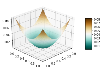
The density accumulates at the boundaries of the distribution’s support. So when we sample, we expect more values around the boundaries rather than the center. The question is how to make our sampling process conforms to the same. In the rest of this post, we will discuss three methods: Rejection Sampling, Gibbs Sampling, Metropolis Hastings.

Rejection Sampling:

The gist of this method is to find a distribution $p(x)$ from which we know how to sample. We scale $p(x)$ by a factor $C$ such that $q(x) \leq C p(x)$

If the above can be obtained, then our sampling procedure is as follows:

Sample $\bar{x}\sim p(\bar{x})$.
Toss a biased coin to accept $\bar{x}$ as a sample coming from $q$. The coin bias is $\frac{q(\bar{x})}{Cp(\bar{x})}$

Intuitvely, you can think of this procedure as a correction scheme to account for the mismatch: how accurately $p(x)$ describes $q(x)$. Put it differently, the area under curve $Cp(x)$ is $C$, while under $q(x)$, it is $1$. And since $q(x)\leq Cp(x)$, if we full the area under $Cp(x)$ with points uniformly, then $1/C$ of these points will be under $q(x)$.

In the demo below, we choose $p$ to be the uniform distribution: $x_1 \sim \mathcal{U}(0,1)$ $x_2 \sim \mathcal{U}(0,1)$ $p(x) = 1$

And $C$ to be $\max_{x} q(x)= 0.0833333$

C = q([0.,0.]) #max_x q(x)
p = lambda x: 1
samples = []
num_samples = 10000
while len(samples) < num_samples:
    x = rnd.rand(2)
    if rnd.rand() <= ( q(x) / (C * p(x))):
        samples.append({'x_1':x[0], 'x_2':x[1]})

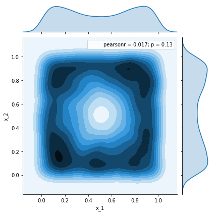
df = pd.DataFrame(samples)
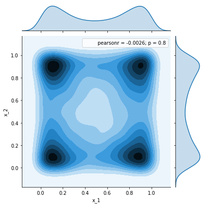
_ = sns.jointplot(x=df.x_1, y=df.x_2, kind='kde')

We can see how the histogram of the collected samples agrees to the mass distribution of $q$. However, this approach becomes challenging in higher dimensions: higher rejection probability $($which makes the process extremely slow$)$ and less known upper-bounding scaled distributions. For this, Markov Chain Monte Carlo $($MCMC$)$ methods come to the rescue

Markov Chain Monte Carlo

Based on the notion of stationary distribution,

$\pi(\bar{x})=\sum_{x}\pi(x)T(\bar{x}|x)$ we can generate our samples from a dynamical systems over the states $($values$)$ which the random variable $x$ can take. That is, i. Specify a transition probability in line with the system dynamics $T(\bar{x}|x)$ $($or proposal distribution- to propose the next state $\bar{x}$ given the present state $x$ $)$. ii. Let the system interact, iii. The system will converge to the underlying $($unique$)$ distribution of $\pi$. Note that, if: $T(\bar{x}|x)>0\;, \forall x, \bar{x}\;,$ there exists a unique stationary $\pi$

The challenge in this setup is how to define / sample from the valid transition distribution $($e.g., in higher dimensions$)$. Among other approaches we discuss two here.

Gibbs Sampling

Given a random $($initialized$)$ state of our systems variables $($here, $x_1$ and $x_2$$)$, one can condition one variable on the other to obtain a 1-D distriubution, which we assume we can sample from $($i.e., rejection sampling, central limit theorem, or other techniques$)$. Iteratively, we will obtain samples. Neverthelss, we need to give it some time till we converge to the stationary distribution of our system. In our example, we will make use of rejection sampling in 1-D to obtain our 1-D sample.


q = lambda x: ((x[0] - 0.5)**2 + (x[1] - 0.5)**2) / 6.
# q(x_1|x_2)
q_1 = lambda x: 6 * q(x)/((x[1]-0.5)**2 + 2. * 0.5**3 / 3.) 
# q(x_2|x_1)
q_2 = lambda x: 6 * q(x)/((x[0]-0.5)**2 + 2. * 0.5**3 / 3.) 
# p (upper bounding), here we are using uniform dist
p = lambda x: 1 

def reject_uniform_sample(q, C):
    while True:
        x_ = rnd.rand()
        if rnd.rand() <= q(x_) /(C * 1.):
            return x_

# aribtrary value, by right we should use max_x q_1, max_x q_2
C_1 = 1.5
C_2 = 1.5
samples = [{'x_1':rnd.rand(), 'x_2': rnd.rand()}]
num_samples = 10000
while len(samples) < num_samples:
    x_1 = reject_uniform_sample(lambda x_: q_1([x_, samples[-1]['x_2']]), C_1)
    x_2 = reject_uniform_sample(lambda x_: q_2([samples[-1]['x_1'], x_]), C_2)
    samples.append({'x_1':x_1, 'x_2':x_2})

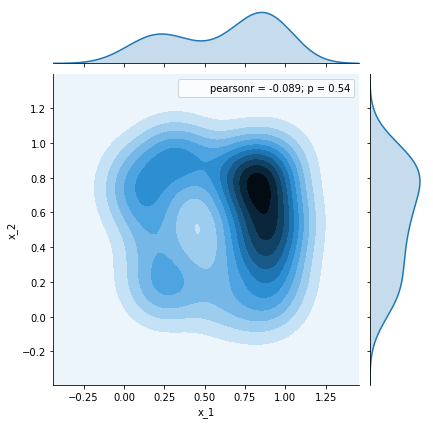
While burning:

df = pd.DataFrame(samples[:50])
_ = sns.jointplot(x=df.x_1, y=df.x_2, kind='kde')

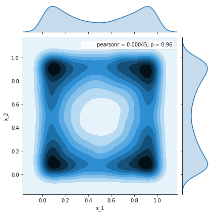
After discarding some samples away:

df = pd.DataFrame(samples[500:])
_ = sns.jointplot(x=df.x_1, y=df.x_2, kind='kde')

Metropolis-Hastings Sampling

In Gibbs sampling, the idea is to generate samples for each of our system’s variables from their posterior distribution with respect to the current values of the rest of the variables. Multi-dimensioanly sampling is reduced into a sequence of 1-D sampling procedures. We saw above, this approach might be a little bit slow and generates highly correlated samples $($again: we are generating samples that are highly probable given the past values of the rest of the variables$)$. Furthermore, what if we can’t compute nor sample from the posterior distribution. Can we propose transitions from one state to another arbitrarily and sitll converge? The idea of MH-sampling is to incorporate rejection sampling with aribtrary proposal distribution such that the transition probability $($which uniquely defines the Markov process$)$ can be constructed.

Let’s step back and summarise the above:

We would like to sample from our system’s distribution $q( x )$ .
We are using Markov Chain $($process$)$ to simulate our system of random variables. That is the Markov chain asymptotically converges to a stationary distribution $\pi(x)$ and which is $q(x)$ .
To converge to $ q(x) $, we need to construct the corresponding chain’s transition probability $ T(\bar{x}|x) $ because it uniquely defines the process and hence its stationary distribution.
One way of achieving that is through the detailed balance, sufficient but not a necessary condition: $ q(x) T(\bar{x}|x) = q(\bar{x}) T(x|\bar{x}) $

We can make use of the above formula to construct a transition probability that is a product of an arbitrary distribution $g(\bar{x}|x)$ , which is referred to as the proposal distribution as mentioned above, and the acceptance distribution $A(\bar{x}|x)$

$T(\bar{x}|x)= g(\bar{x}|x)A(\bar{x}|x)$

Plugging this in the detailed balance condition, we have:

$A(\bar{x}|x)=\min\{1, \frac{q(\bar{x})g(x|\bar{x})}{q(x)g(\bar{x}|x)}\}$

Let’s see how we can realize this in code: Let’s define our

$g(\bar{x}|x)\sim \mathcal{N}(x,0.25I)$

and here we are assuming that we can sample efficiently from this 2-D Gaussian distribution $($ otherwise, we may use one of the techniques above as rejection sampling $)$. Notice here, there is nothing preventing us from sampling outside the support of $q(x)$, so we need to explicitly state that. I.e., $q(x)=0$ outside $q$’s support. Also, our choice of proposal distribution might affect the convergence progress.

# target distribution (the one we'd like the MC to converge to)
q = lambda x: ((x[0] - 0.5)**2 + (x[1] - 0.5)**2) / 6.
# assuming 2-d Gaussian sampling is doable here (via function call)
sigma = 0.5
propose_x = lambda x_prev: x_prev + sigma * np.dot(rnd.randn(1,2),np.eye(2))[0,:]
# proposal distribution:
from scipy.stats import multivariate_normal
g = lambda x_new, x_prev: multivariate_normal.pdf(x_new, mean=x_prev, cov =sigma * np.eye(2))
# random initialization of the sample which we'll eventually discard
samples = [{'x_1':rnd.rand(), 'x_2': rnd.rand()}]
num_samples = 10000
while len(samples) < num_samples:
    x_prev = np.array([samples[-1]['x_1'], samples[-1]['x_2']])
    x_new = propose_x(x_prev)
    # to discard samples out of support
    if max(x_new) > 1. or min(x_new) < 0.:
        continue
    if rnd.rand() <= min(1, q(x_new) * g(x_prev,x_new) / (q(x_prev) * g(x_new, x_prev))):
        samples.append({'x_1':x_new[0], 'x_2':x_new[1]})

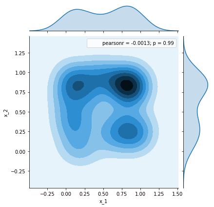
df = pd.DataFrame(samples[:50])
_ = sns.jointplot(x=df.x_1, y=df.x_2, kind='kde')

df = pd.DataFrame(samples[1500:])
_ = sns.jointplot(x=df.x_1, y=df.x_2, kind='kde')