A Practical Summary to Matrix Inversion

$ \newcommand{\vx}{\mathbf{x}} \newcommand{\vq}{\mathbf{q}} \newcommand{\vb}{\mathbf{b}} \newcommand{\lm}{\lambda} \newcommand{\norm}[1]{||#1||_2} \newcommand{\mat}[1]{\left[#1\right]} $

Matrix inversion is a handy procedure in solving a linear system of equations based on the notion of identity matrix $I_n\in\mathbb{R}^{n^2}$ whose all entries are zero except the entries along the main diagonal.

For a linear system $A\vx=\vb$ where $A\in\mathbb{R}^{m\times n}$ is a known matrix, $\vb\in\mathbb{R}^m$ is a known vector, and $\vx\in\mathbb{R}^n$ is a vector of unknown values, one can find a solution if a matrix $B\in\mathbb{R}^{n\times m}$ can be found such that $BA=I_n$ since for all $\vx \in \mathbb{R}^n$, $I_n \vx=\vx$. We refer to $B$ as the inverse of $A$ $($commonly denoted as $A^{-1})$. Mathematically,

$$A\vx=\vb$$ $$A^{-1}A\vx=A^{-1}\vb$$ $$I_n\vx=A^{-1}\vb$$ $$\vx=A^{-1}\vb$$

Of course, such solution can be found if $A$ is invertible. That is it is possible to find $A^{-1}$. I am writing this post to summarize possible scenarios one may face when inverting a matrix.

Before delving into the details, I intend to present a geometric view of linear systems of equations. This will help us understand why we could have exactly one, infinitely many, or no solution at all. And subsequently, why some matrices are invertible and others are not.

Problem Setup

One can think of $\vb$ as a point in the $m$-dimensional space. Furthermore, consider $A\vx$ as a linear combination $A$’s column vectors where the $i^{th}$ column $A_{:,i}$ is scaled by the $i^{th}$ entry of $\vx$, $x_i$. In other words, when we say that $\vb=A\vx$, we mean that $\vb$ is reachable from the origin $(\mathbf{0}\in\mathbb{R}^m)$ by moving $x_1$ units along the vector $A_{:,1}$, $x_2$ units along the vector $A_{:,2}$, …, and $x_n$ units along the vector $A_{:,n}$. For different $\vx\in\mathbb{R}^n$, we may reach different points in the $m$-dimensional space. The set of such points are referred to as the span of $A$ $($or range of $A$, column space of $A)$. That is, the set of points reachable by a linear combination of $A$’s columns. Mathematically, $span(A\text{'s columns})=\{b\in \mathbb{R}^m|\; b = A\vx,\; \vx\in \mathbb{R}^n\}\;.$

Therefore, a solution exists for $A\vx=\vb$ if $\vb\in span(A\text{‘s columns})$. A necessary and sufficient condition for a solution to exist for all possible values of $\vb$ $(\mathbb{R}^m)$ is that $A$’s columns constitute at least one set of $m$ linearly independent vectors. Let’s note that there is no set of $m$-dimensional vectors has more than $m$ linearly indepdent vectors. The following examples provide an illustration.

1. $A=\mat{\begin{array}{cc} 1 & 2 , 0 & 0\end{array}}$, $\vb =\mat{\begin{array}{c} 1 , 1\end{array}}$. In this example, $A$’s span is $\mathbb{R}^1$ along the vector $\mat{\begin{array}{c}1 , 0\end{array}}$ and no matter how $\vx$ is set, we can not reach $\vb$, because it does not lie at the intersection of its plane $\mathbb{R}^2$ and $A$’s space. With regard to the remark made above, we notice that $m=2$, but we do not have $2$ linearly independent vectors in $A$’s columns.
2. $A=\mat{\begin{array}{cc} 1 & 2 , 0 & 0\end{array}}$, $\vb =\mat{\begin{array}{c} 1 , 0\end{array}}$. In this example, $A$ is the same as $(1.)$’s but we moved $\vb$ to make it reachable. One may note that the effective dimension of the problem at hand is one (the second entry of all the columns is zero). In other words, we have matrix of $1\times 2$ with $m=1$ and we have $2$ linearly dependent vectors of length 1 that can reach $\vb$ through any solution that satisfies $x_1+ 2x_2=1$, for which there are infinitely many. Such example fulfills the sufficient and necessary condition aforementioned, but here we have more than $m$ columns. Thus, there are infinitely many solutions rather than exactly one.
3. $A=\mat{\begin{array}{cc} 1 & 0 , 0 & 1\end{array}}$, $\vb =\mat{\begin{array}{c} 1 , 1\end{array}}$. In this example, we made $A$ spans $\mathbb{R}^2$ with exactly $m=2$ linearly indepdendent vectors, and so we can reach $\vb$ with exactly one particular $\vx$. This example fulfils the sufficient and necessary condition with exactly $n=m$ columns.

Based on the above, one can conclude the following:

1. When $A$ is a square matrix $(m=n)$ with $m$ mutually independent column vectors, there is exactly one solution for any $\vb\in\mathbb{R}^{m}$. Thus, $A$ is invertible.

2. When $A$ is a square matrix $(m=n)$ with linearly depdenent column vectors, there exists some $\vb$ for which no solution exists. Thus, $A$ is non-invertible and we say that $A$ is a singular matrix.

3. When $A$ is a rectangular matrix $(m>n)$, there exists some $\vb$ for which no solution exists. Thus, $A$ is non-invertible, and we say that the system is overdetermined.

4. When $A$ is a rectangular matrix $(m< n)$ with $m$ linearly indendent column vectors, there exist infinitely many solutions for any $\vb \in \mathbb{R}^m$. Thus, $A$ is non-invertible, and we say that the system is underdetermined.

5. When $A$ is a rectangular matrix $(m< n)$ with $< m$ linearly indendent column vectors, it is possible that there exists some $\vb$ for which no solution exists. Thus, $A$ is non-invertible. We still say the system is underdetermined.

There are several procedures to compute $A^{-1}$ for invertible matrices such as the Gauss elimination method $($some others are listed in the figure at the bottom of this page$)$.

Non-Invertible Matrices

So what do we do when $A$ is non-invertible and we are still interested in finding a solution for a system? Well, we can use a pseudo-inverse matrix with some compromise on the solution’s quality as follows.

• If there is no solution. That is we can’t reach $\vb$ and the system is overdetermined. Then, we can choose one with the least squares error. Mathematically,

$$\min_{\vx} ||A\vx-b||^2_2$$

Differentiating w.r.t $\vx$ and setting it to zero,

$0=\nabla_{\vx}{((A\vx-b)^{T}(A\vx-b))}=A^{T}A\vx-A^T\vb$ yields $\vx=(A^{T}A)^{-1}A^T\vb$. Therefore, the pseudo-inverse matrix is $(A^{T}A)^{-1}A^T$

• If there are infinitely many solutions. That is the system is underdetermined. Then, one can choose one with the minimum norm. Mathematically,

$\min_{\vx} ||\vx||^2_2$ $\text{s.t.}\;\;\; A\vx =\vb$

With the Lagrangian multipliers trick, the above can be solved as follows.

Differentiating w.r.t $\vx$ and setting it to zero,

$$0=\nabla_{\vx}{(\vx^{T}\vx - \mathbf{\lambda}^{T}(A\vx-b))}= 2\vx - A^{T}\mathbf{\lambda}$$

$A^{T}$ is not invertible, but $AA^{T}$ is.¹ Therefore, we can solve for $\mathbf{\lambda}$ as follows.

$$\mathbf{\lambda}= 2(AA^T)^{-1}A\vx=2(AA^T)^{-1}\vb$$

Thus, $\vx=A^T(AA^T)^{-1}\vb$

Interestingly, both of the above pseudo-inverses are equivalent to the Moore-Penrose pseudo-inverse which can be computed from the singular value decomposition $($SVD$)$.

Ill-Conditioned Matrices

Let’s motivate this issue with an example. Assume you are reading a measurement, which you have to scale by dividing by a very small number. If your reading deviates a little, the absolute error will extremely large. Such large oscillations might be undesirable and we’d like to dampen them. In the matrix world, dividing by a small number corresponds to to multiplying by the inverse of an ill-conditioned matrix. An ill-conditioned matrix is still invertible, but it is numerically unstable. In addition to the measurement error $($here the measurement is captured by $\vb$$)$, inverting an ill-conditioned matrix also suffers from loss of precision in floating point arithmetic.To cope with this unstability, we compromise the quality of the solution and use regularization techniques to have a stable numerical outcome. The bulk of these techniques aim to increase $($or replace$)$ the value of the smallest eigenvalue with respect to the greatest eigenvalue. Common techniques are:

1. Truncated SVD
2. Tikhonov Regularization $($which can also be used for non-invertible matrices$)$.

It is important to consider the regularization effect on the final solution and whether it makes sense to our system or not.

Matrix Inversion Summary

Below is a summary on matrix inversion.

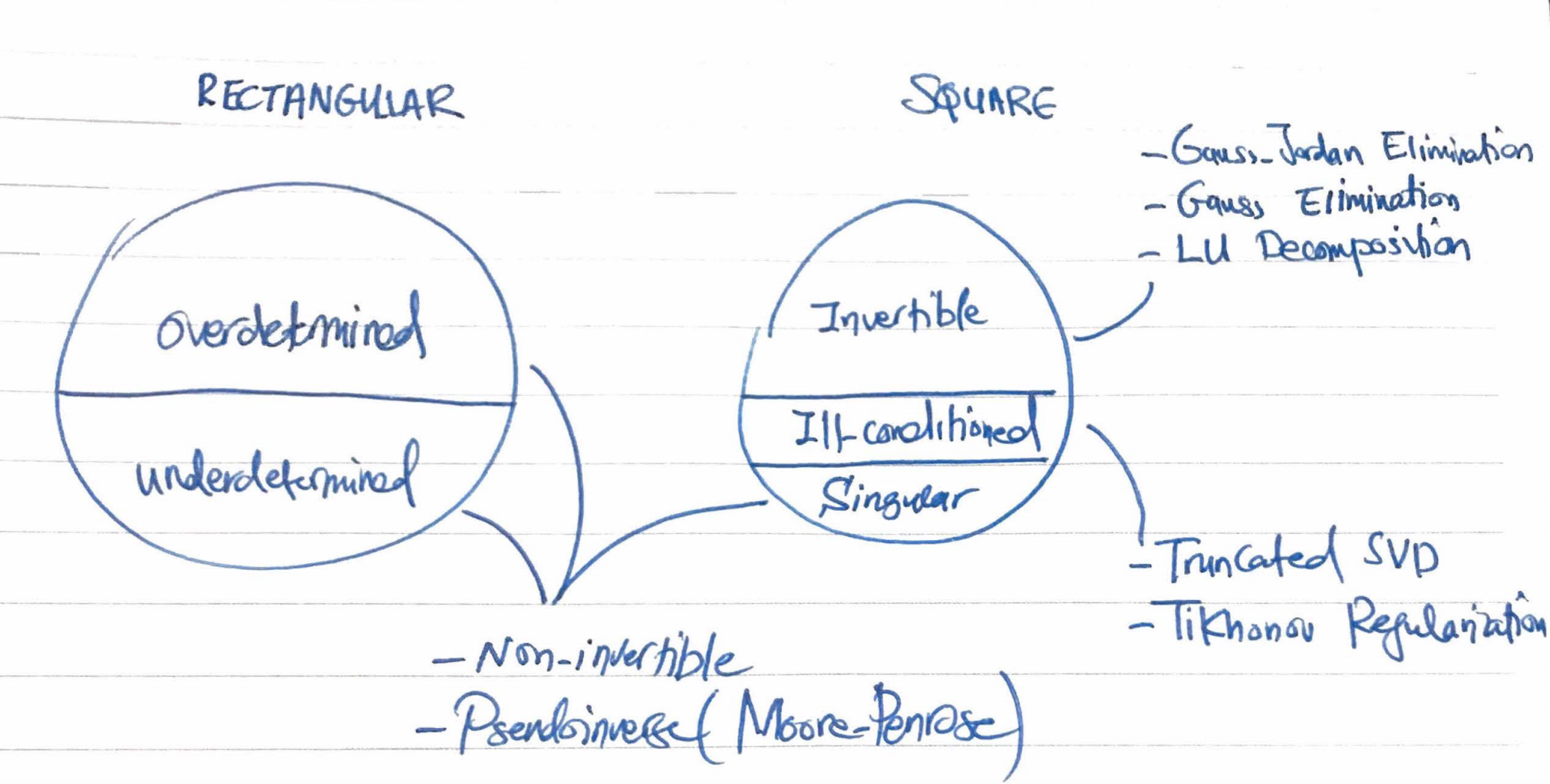
Summary of Matrix Inverse Techniques.