Random Projections for Lipschitz Functions
In this post, we’ll shed some light on the behavior of Lipschitz-continuous functions at random projections of the same point in another space. Consider Figure 1; we have a point in the $\mathbf{y}$ in the lower dimensional space $\mathcal{Y}$ that is projected randomly to the higher dimensional space $\mathcal{X}$ twice using two randomly sampled matrices $A_p$ and $A_q$. With this setting at hand, we are interested in the following question: is there a relation between the function values at $A_p\mathbf{y}$ and $A_q\mathbf{y}$. This has been addressed in [1, Theorem I]. Here, we provide a numerical validation of [1]’s result besides reiterating the formal proof. Before we delve into this further, let’s introduce some notation in accordance with [1].
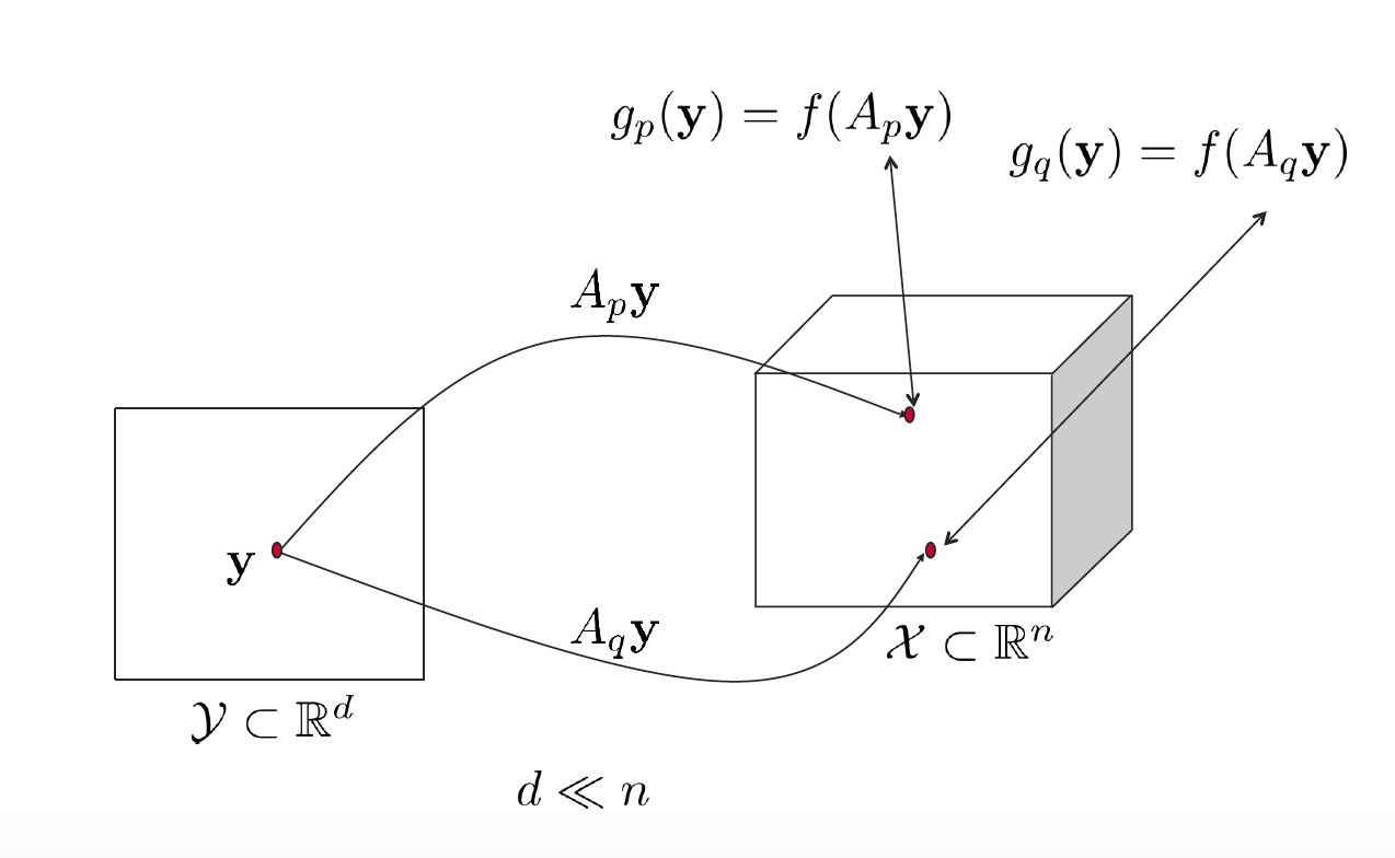
Figure 1. Two random projections of $\mathbf{y}$ to $\mathcal{X}$.
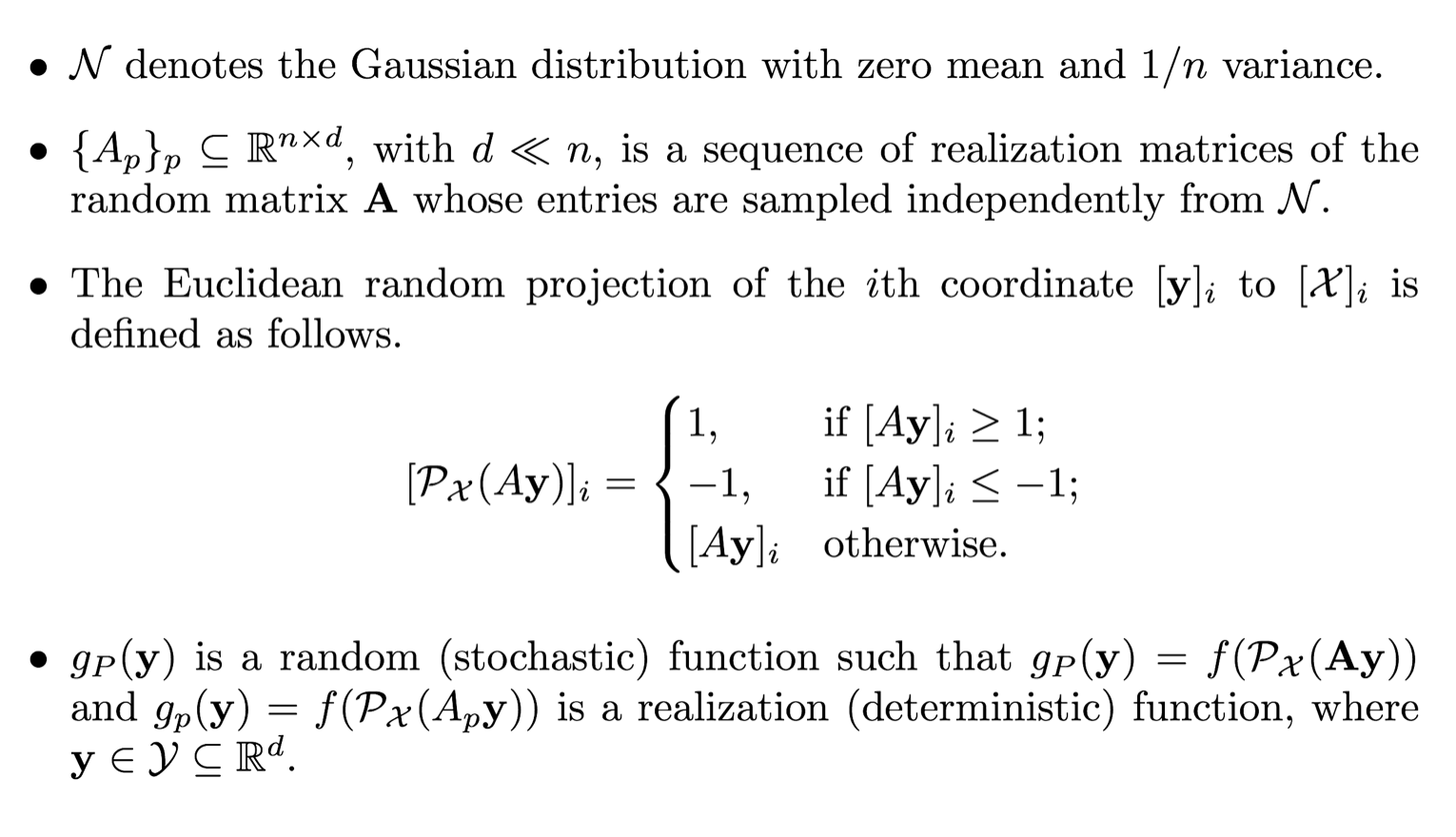
Notation
Theorem I [1]
It has been shown in [1] that the mean variation in the objective value for a point $\mathbf{y}$ in the low-dimensional space $\mathcal{Y} \subset \mathbb{R}^d$ projected randomly into the decision space $\mathcal{X}\subset\mathbb{R}^n$ of Lipschitz-continuous problems is bounded.
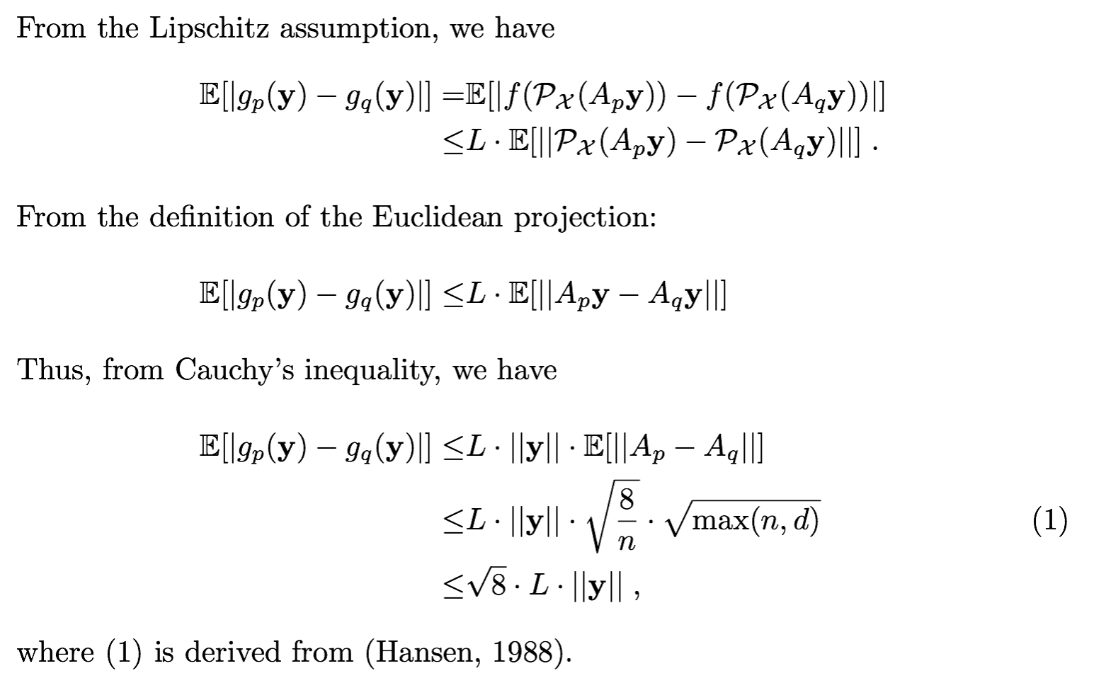
Mathematically, for all $\mathbf{y} \in \mathcal{Y}$, we have
Here, we reproduce [1]’s proof for completeness, then we validate the theorem numerically.
Proof
Numerical Validation
Here, we carry out a numerical validation of [1]’s Theorem I over four popular Lipschitz-like benchmark functions $($namely, Cigar, Sphere, Rastrigin, and Bohachevsky$)$.
First, we sampled 100 points $\mathbf{y}\in\mathcal{Y}\subset \mathbb{R}^d$ whose norms span the range $[0,1]$. E.g., with $d=1$, $\mathbf{y}\in[-1,1]$.
Second, each of these 100 points are projected to the function space $\mathcal{X}\subset\mathbb{R}^n$ using 20 random matrices ${A_p}_{1\leq p\leq 20}$.
Third, the four considered functions are evaluated at these random projections. Note that for each of these functions, $100*20$ function evaluations are performed.
Fourth, we average over the absolute difference between function values at projections of the same point $\mathbf{y}$. That is, for each of the 100 points, we compute the mean of $\frac{20*20- 20}{2}=190$ values, each of which representing the absolute difference of the function value at two random projections of the corresponding point $\mathbf{y}$.
Fifth, the computed average values are plotted as a function of the corresponding point $\mathbf{y}$ in Figure 1. One can see how the trend of the plot follows the curve of $||\mathbf{y}||$ in accordance with [1]’s Theorem I.
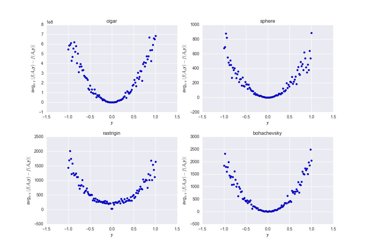
Figure 2. Empirical mean of the absolute value difference of four functions evaluated at 20 random projections in $\mathbb{R}^n$ of a point in $\mathbb{R}^d$, where $d=2$ and $n=10^3$.
References
This post is based on the following papers:
- Al-Dujaili, Abdullah, and S. Suresh. “Embedded Bandits for Large-Scale Black-Box Optimization.” Thirty-First AAAI Conference on Artificial Intelligence. 2017.